Thesis Eric Groen Chapter 1

During head movements, the vestibular system generates compensatory eye movements for stabilization of the retinal image. In the case of head rotation about the roll-axis, this results in rotation of the eyes about the visual axis, generally referred to as ocular torsion (OT). The sustained OT response to static tilt of the head is attributed to stimulation of the otolith organs (Cheung et al. 1992; Miller 1962; Miller and Graybiel 1971; Woellner and Graybiel 1959), whereas OT during dynamic head tilt is primarily generated by the semicircular canals (Collewijn et al. 1985). Non-vestibular inputs, however, such as proprioception from the neck, may contribute as well (De Graaf et al. 1992). In addition to the field of basic research, OT measurement may also find clinical applications in the field of oto-neurology (Diamond and Markham 1981; Dieterich and Brandt 1993 Gresty and Bronstein 1992).

Several techniques for OT determination have been described, varying from photographic procedures (Miller 1962; Graybiel and Woellner 1959; Melvill Jones 1962), to the semi-invasive and accurate search coil method (Robinson 1963; Collewijn et al. 1985). Expanding on photographic methods, advanced video-based techniques offer great flexibility: the approach is non-invasive, no calibration is needed and images are directly available for analysis. Like photographic methods, video-based techniques commonly measure OT by tracking iris structures. Hatamian and Anderson (1983) described an algorithm for OT measurement in digitized video images based on cross-correlation of a sampled iris pattern encircling the pupil. Such an algorithm was implemented in automatic methods developed by Clarke et al. (1989) and Bucher et al. (1990). The apparatus of Clarke et al. allowed for analysis of the vestibulo-ocular reflex in all directions: vertical and horizontal gaze direction on-line, and OT off-line.

Recently, Bos and De Graaf (1994) introduced a semi-automatic method for OT quantification, especially designed for the correction of errors that arise from incorrect assessments of the pupil center (which is assumed to coincide with the rotation axis of the eye). It was shown that this type of error varies sinusoidally in tangential direction and may amount to 1-2º, which is sometimes on the order of OT itself. By averaging OT values determined in opposite segments of partitioned annular iris strips, this type of error can largely be corrected for, yielding a practical accuracy of about 0.25º. In the implementation of this method, OT determination was carried out by matching iris patterns visually on a computer monitor. Consequently, the method was appropriate for static OT measurements, involving a small number of images, but not very efficient for OT measurements under dynamic conditions, involving larger series of images. Therefore a fully automatic system was developed which made use of the error analysis of Bos and De Graaf. As a prerequisite, the method should take as many as possible iris segments into account for a reliable estimate of OT. A procedure of tracking 36 distinct landmarks, well spread over the iris, was considered appropriate for this purpose. An algorithm for template matching was derived from In den Haak et al. (1992) which allows for automatic selection and relocation of the most salient iris structures in two directions. The procedure and its implementation will be described in this chapter. The system's reliability will be evaluated in both an in vitro and an in vivo study. The results show that two-dimensional template matching is an useful alternative for the common one-dimensional cross-correlation between iris strings.

Figure 1.1. The head set with one lipstick CCD-camera (another camera can be mounted in front of the other eye). The aluminum frame allows for careful adjustments of the camera.

The system hardware consists of two small CCD-cameras mounted on a pair of diving goggles (Figure 1.1). The cameras are placed in front of the eyes at a distance of about 1-2 cm, the optical axes aligned with the visual axes. Each eye is illuminated by a small white light emitting bulb, closely fixed to the camera. To avoid artifacts by movement of the headset relative to the head, the headset can be attached to a dental frame. Both eyes are recorded separately on S-VHS tape, mixed with an analogue time code signal for synchronization. For off-line analysis, the video recorder (Panasonic AG-6730) is controlled by an RS232-interface protocol. Recordings are made using European video standard PAL (25 frames/s, each frame consisting of two interlaced fields). By playing one field at a time, a temporal resolution of 20 ms is realized. The fields are digitized into 512*512 pixel images with a depth of 8 bits by a PC-Vision Plus frame-grabber (Imaging Technology Inc., Bedford, MA).

Figure 1.2. Schematic representation of the total procedure. In a reference image, the pupil is identified, and a ring-shaped iris area is selected and converted into polar coordinates (so that it projects on a rectangular grid). After gray value normalization, the iris area is divided tangentionally in 36 segments of 10º, in each of which one landmark is selected. These landmarks then are relocated in the corresponding iris areas in consecutive data images.

The OT determination is based on tracking a set of distinct landmarks in the iris in a number of data images relative to one reference image (Figure 1.2). In the analysis, six steps can be identified: 1) pupil detection, 2) polar transformation, 3) normalization, 4) selection of significant points, 5) matching, and 6) OT estimation.

The software automatically determines the pupil center, which is assumed to lie on the axis of rotation. The pupil is the largest dark area in the image and is separated from the surrounding iris by simple thresholding at a value just beyond the first clear peak in the gray value distribution. Eventually, some additional smaller dark regions, like eyelashes or shadows, remain after thresholding and the pupil is distinguished from these by connected area labeling (Sedgewick 1984).

To obtain the center of rotation, the imaged pupil edge is approximated by a circle (the subject is looking straight into the camera). To compute the parameters of the circle (center (x₀ ,y₀), and radius R), we applied the method of Chaudhuri and Kundu (1993). This method is based on minimizing the least square error J, with

(where the summation is over all edge points (x_i , y_i) with i = 1..n). This can be done by setting the derivative of J with respect to x₀, y₀, and R to zero. Then x₀, y₀, and R are given by:

Figure 1.3. Despite deformations of the pupil edge, caused by reflection artifacts and a partial eye blink, the pupil has been localized successfully by means of a reweighted least squares circle approximation to the edge points. The raw thresholded pupil edge is marked by the frayed line, whereas the fitted circle is shown as the thick solid line.

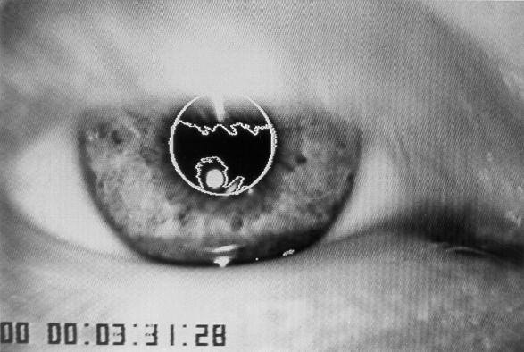
Figure 1.4. Weights w_i are assigned to the pupil edge points according to their distance ½ d_i½ to the previous circle fit, expressed in terms of the standard deviation of these distances (s _n-1). Dubious edge points with a distance ½ d_i½ of more than 2s are excluded by setting the weight to zero.

Illumination artifacts and eyelids may cause deformations of the imaged pupil edge (Figure 1.3). The influence of these artifacts on the analysis can be reduced by giving dubious edge points low weight values w_i. Initially, it is not known which edge points are dubious, and all weights are set to unity. Then, all edge points are reweighted depending on their deviation from the fitted circle, and the calculation of x₀, y₀ and R is repeated. The most natural choice for the weights is the reciprocal of the squared distance from the individual points (x_i , y_i) to the previously fitted circle, i.e. w_i = 1/d_i² with d_i =

. It is even better to exclude points that clearly do not belong to the true pupil edge completely. An appropriate weighing, as depicted in Figure 1.3, is then given by w_i = 1-d_i/(2s ) for ½ d_i½ < 2s , and w_i=0 otherwise, where the overall standard deviation s is considered explicitly (s ²=å d_i²/(n-1)). This procedure of fitting and weighing is executed eight times.

Once the center and radius of the pupil have been determined, an annular iris area of fixed width is selected (Figure 1.5A). The distance of this iris ring to the pupil border can optionally be adjusted in the reference image to overcome reflection artifacts. Once chosen, the distance to the pupil border is invariable for all consecutive data images, so that the same iris area will be selected automatically, irrespective of expansion or constriction of the iris due to variations in pupil size. After Gaussian smoothing to avoid aliasing, the selected region is transformed into polar coordinates, so that it is represented on a rectangular grid (Figure 1.5B): rotation (OT) in the original image then corresponds with translation in the converted image (translation is computationally less expensive).

Let (r,f ) denote the polar coordinates to which the points of the selected iris region will be projected, r being the radius and f the azimuth angle of each point, and (x₀ ,y₀) be again the center of the pupil in Cartesian coordinates. Then the relation between the transformed image I(r,f ) and the original image F(x,y) is determined as follows:

The angle f is quantized into 0.25º bins (rounded to the nearest pixel index), and the radial extent of the annulus is sampled in 39 steps, which covers nearly half of the iris width. Finally, the iris strip projects on a rectangle of 39x1440 bins (hereafter treated as pixels again).

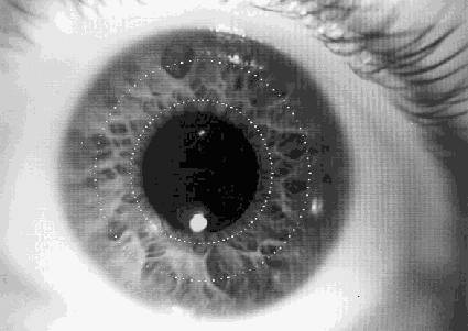
Figure 1.5a. Selection of the area of interest. After the pupil center and radius have been estimated, an annular band of fixed width is selected around the pupil (between dotted circles). The distance between this band and the pupil edge can be adjusted manually in the reference image, and will be held constant for all data images.

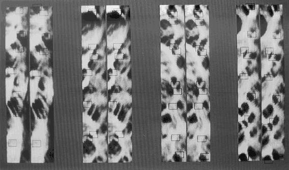
Figure 1.5b. After transformation into polar coordinates the annular iris band is represented by a rectangle. Here the rectangles of both a reference (left) and a data image (right) are shown of real eyes. For practical reasons the rectangles are displayed in 4 segments of 90º. Adjacent segments correspond with respect to their position in Cartesian coordinates. OT is calculated by the translation of 36 landmarks (square masks) between these rectangles. OT is -0.9º in this example.

Although great care is taken to guarantee constant illumination of the eye, the use of a small light bulb may result in an illumination gradient (Figure 1.5A). Luminance differences can also occur, e.g., by reflections from the headset. To eliminate these luminance differences between images and to facilitate relocation of significant points, two procedures are applied on the polar transformed iris images. First, the gradient that occurs with radiant illumination is largely removed by a high-pass moving average filter covering 40º, moving unidirectional along f , and effectively eliminating structures larger than 63º (c.f. Faes et al. 1994). Second, by means of a parameter-free histogram equalization, gray values are stretched to include the entire gray scale, with exception of the maximum gray value. The latter is reserved for identification of reflections, defined as pixels with original gray values above the 80^th percentile of the gray scale. In the following analysis reflection areas will be excluded. Because the same iris area is selected in all images, this normalization procedure will equalize gray values of corresponding structures.

In the iris of the reference image, significant points are selected which are to be recognized in successive data images. A suitable method to find unambiguous patterns was presented by In den Haak et al. (1992). Their method selects points at junctions of distinct dark and bright structures (Figure 1.6). Following a path along the sides of a small square (a "mask", typically between 10*10 and 20*20 pixels) centered at those points, the number of times the gray value increases or decreases is counted (Figure 1.7). To be independent of noise, gray value transitions must exceed a certain noise level. We chose the noise level to be the standard deviation of gray values of the entire iris strip (which is a constant after the normalization step). The significance of a mask is defined as the number of gray value transitions greater than this noise level. We chose a mask size of 15*15 pixels, which is in correspondence with the general size of the iris patterns as can be judged from Figure 1.4b. To achieve a fairly homogeneous distribution of landmarks, the iris is divided into 36 sectors of 10º each, and for each sector the most significant structure is determined. Masks which cover a reflection are ignored.

2) For an optimal histogram equalized image with gray values Ii in the range [0,m] and i in [1,N], each I occurs exactly n = N/m times, and the average gray value I=½ m Then

Figure 1.6. This drawing shows that a mask covering a multiple ramification of iris structures (b) can be successfully relocated because the precise location of gray value transitions under the mask prevent it to move in any direction, as opposed to a mask covering a more ambiguous structure such as an edge (a).

Figure 1.7. The calculation of the significance of a mask. Following the gray value profile along the sides of the mask, the number of gray value transitions that exceed the noise level, are counted. The counted transitions here are a, b, d, and e. The "up" transition c is ignored, because it is followed by another "up" transition. (after: In den Haak et. al. (1992), by kind permission).

Significant structures from the reference image are recognized in the data image by template matching. Let M denote the border of a 15x15 square mask, centered at some point in an iris image. Let I_u and I_v denote the gray values of the iris of the reference image and data image iris respectively, as defined in equation 1. Then the match error, E, for a significant point u=(r_u ,f _u) in the reference image and a point v=(r_v ,f _v) in the data image, is defined as

This match error is simpler and computationally faster than the normalized cross-correlation used by In den Haak et al. (1992). It is permitted because gray values of corresponding iris structures in reference and data images have been normalized beforehand by the histogram stretch. Furthermore, as a consequence of the transformation to polar coordinates, iris structures retain their orientation in spite of changing torsion angle.

For each point u in the reference image, a point v in the data image is determined for which E is minimal. The difference in f -coordinates D F =f _v-f _u of each pair yields a measured torsion angle. In this way, up to 36 D F -values are obtained. To reduce analysis time, searching is restricted to intervals of D F between ±25º, since OT never exceeds this range.

In determining the true torsion angle from these measurements, two problems arise. First, mismatches should be excluded from the estimation process. Second, as indicated by Hatamian and Anderson (1983) and Bos and De Graaf (1994), misalignment of the pupil center with the true rotation center results in a measured torsion angle, D F , that varies sinusoidally with the angular position f of the landmark around the rotation center (Figure 1.8). The same problem occurs when the imaged pupil shape is not circular, due to gaze shifts with respect to the camera position. We can thus characterize the estimation problem as a sinusoidal fit, eventually corrupted by outliers. Analogous to the circle fit procedure in the pupil detection, we apply an iterative reweighted least squares approximation to the measurements (f _i ,D F _i), i=1..36 (see e.g. Hogg 1979):

The method was implemented on a PC (Intel 486, 66MHz), in which the analysis took about 7 s per image: digital image processing needed 4 s, where the remaining time was consumed by operation of the video recorder, and storage and displaying of the results.

Figure 1.8. Robust estimation of OT from individual determined torsion angles. The 36 measured torsion angles (squares) depicted against the angular position in the iris (f ) of the corresponding landmarks. Misjudgment of the rotation center results in a sinusoidal variation of the measured torsion angles about OT. Therefore, a robust sinus fit procedure is applied on the measurements to estimate OT. In this figure OT amounts to -3.0 deg.

The accuracy of the automatic system was first validated using the same set of prepared images of an artificial eye as was used by Bos and De Graaf. The torsion angle of this artificial eye could be set with an accuracy of 0.1º. The torsion angle was varied in steps of 5º from -10º to +10º, and the angle between the line of sight and the camera's optical axis was either 0º or 10º. In this way, ten data images were prepared. The error in the computed OT for each image is shown in Figure 1.8. At the most, this error was 0.11º, i.e. on the order of the precision of the setting of the artificial eye itself.

Figure 1.9. The error in automatically reproduced torsion angles in ten images of an artificial eye. The squares and triangles denote that the camera-visual axis was 0º (axial) and 10º (non-axial), respectively.

Second, the system was validated by applying it to a set of 256 images of real eyes obtained from 8 different subjects who had been positioned at various angles of lateral body tilt. The system's reliability was evaluated by comparing the automatically determined OT values with the results of three examiners who used the semi-automatic method Bos and De Graaf (1994), which served as a reference. Figure 1.9 shows that the results of both methods are in close agreement for the entire series of observed torsion angles from -11.4º to 8.9º (for graphical representation, the data have been sorted according to the mean of the OT values estimated by the three examiners). Comparing the system’s value with the examiners' average, the inter-examiner variability should be taken into account. In 94% of the images, the difference between the automatically computed torsion angles and the examiners' average was within two times the examiners' standard deviation (s _n-1). In the remaining 6% of the images, the automatic system failed to find a reasonable match, resulting in a difference with the examiners' average of 1º or more (Figure 1.10). This increased variability could be attributed to inadequate focusing in these specific images, caused by large gaze shifts of the eye with respect to the camera. In most of these cases, the inter-examiner variability exceeded the practical accuracy of the semi-automatic method (0.25º) as well.

Figure 1.10. Validation results with images of real eyes. OT was estimated by both the automatic system and three examiners using the semi-automatic system. The images have been sorted by the examiners' average. The automatically computed OT values are depicted by dots, whereas the results of the semi-automatic method are shown by the examiners' average plus and minus the standard deviation (upper and lower solid line, respectively).

In conclusion, these results demonstrate that the automatic system determines OT in an accurate and reliable way. Based on the overall correspondence with the semi-automatic method, we conclude that with real human eyes, the practical reliability of the system is 0.25º. The performance of the automatic system does not depend on the amount of torsion itself. Coincidental mismatches can be detected as outliers in time-series analysis because of the coherence of such an OT signal.

Automated video-based techniques described previously quantify ocular torsion with cross-correlation of a narrow circular sampled iris pattern (Clarke et al. 1989; Bucher et al. 1990). The method presented here uses an alternative strategy by tracking a set of 36 landmarks, uniformly distributed over a wide annular iris strip. As a result, the method is robust with respect to variations in pupil size, and it enables correction for systematic errors due to misdefined pupil centers. Another important feature of the system is that it autonomously selects landmarks as areas of high interest, facilitating the relocation in the data images. Applied in this way, pattern recognition by template matching is an effective tool for automatic determination of ocular torsion. Although not real-time, the analysis is performed automatically (hands-free) and considerably faster than the semi-automatic method described by Bos and De Graaf (1994).

Because In den Haak et al. (1992) applied their algorithm of template matching in Cartesian coordinates, the masks became distorted by rotation of the image, thereby reducing the match performance. This problem does no longer exist in polar coordinates. This was demonstrated by the consistency of the OT measurements through a wide range of torsion angles in the validation studies.

To assess the accuracy of an OT measurement technique explicitly, the torsion angle should be known. This was the case in the in vitro study with an artificial eye, and the automatic system reproduced the torsion angle accurate to 0.1º. The question whether the results are reliable in a practical sense was addressed by an in vivo validation study taking real human eyes into consideration. Apart from some mismatches, the computed results were indistinguishable from those of the reference method with a general variability of 0.25º. This observation concerns individual images, and may be improved by time-series analysis. Mismatches can be recognized as outliers and rejected by postprocessing. Consequently, also in static conditions it is preferable to analyze a series of consecutive images, rather than a single snap shot, to avoid the risk to rely on a coincidental mismatch.

This study was financially supported by the Foundation for Behavioural and Educational Sciences of the Netherlands Organization for Scientific Research. The authors are indebted to Mr. J. Varkevisser, Mr. L.W.M. Spiekman, and Dr. S. De Vries for their support.

Intro	Chap. 1	Chap. 2	Chap. 3	Chap. 4	Chap. 5
Summary	Concl. Remarks	Bibliography	Samenvatting	CV	Publications